How to describe a system by a Markov process
fiabilipy enables the users to model a system trought a Markov process. This tutorial aims to introduce how fiabilipy handles the Markov modelisation. This introcduction is done using a example.
Let’s say we have a parallel-series system, represented by the following figure.
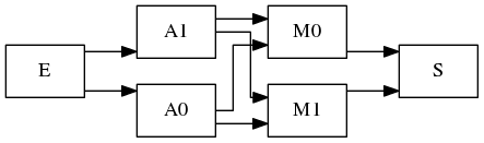
A parallel-series system
We are interested by the probabilities for the system to be :
- in normal state (i.e. every component works)
- in damaged state (i.e. one or more component don’t work, but the system does work)
- in faulty state (i.e. the system doesn’t work at all)
- in available state (i.e. the system is not faulty)
Compoment and process initialisation
To begin, let’s start building the components:
>>> from fiabilipy import Component, Markovprocess
>>> A0, A1 = [Component('A{}'.format(i), 1e-4, 1.1e-3) for i in xrange(2)]
>>> M0, M1 = [Component('M{}'.format(i), 1e-3, 1.2e-2) for i in xrange(2)]
>>> components = (A0, A1, M0, M1)
To initialize the process, we need to give to fiabilipy the list of the components and the initial states probabilities. A state is defined by a number which, in base 2, says if the ith component is working or not. So, with 4 components, we have \(2^4 = 16\) possible states. The following table represents the possible stats (W stands for working and N for not working).
| state | A0 | A1 | M0 | M1 |
|---|---|---|---|---|
| 0 | W | W | W | W |
| 1 | W | W | W | N |
| 2 | W | W | N | W |
| 3 | W | W | N | N |
| … | … | … | … | … |
| 15 | N | N | N | N |
Now, let’s assume that, at \(t = 0\), the probabilities of the system to be in state 1 is 0.9 and state 2 is 0.1, thus we have:
>>> initstates = {0: 0.9, 1:0.1}
>>> process = Markovprocess(components, initstates)
Working states definition
Now we have initialized our Markov process, we have to define the states to be tracked. This is done a writing a function which return True if the given state is tracked False otherwise. The functions will be called with one argument, let’s say x. This variable is a boolean array, the ith case is True if the ith component is currently working, False otherwise.
Ok, let’s define the states we want to track.
Normal state
In this state, every component has to work. So, in python is can be written as:
>>> def normal(x):
...     return all(x)
This function returns True if every single item of x is True.
Available state
In this state, the system is available. So, there exists a path of working components for E to S. That is to say either A0 or A1 are working and M0 or M1 are. So, the function describing the faulty state may be:
>>> def available(x):
...     return (x[0] or x[1]) and (x[2] or x[3])
Damaged state
Actually, when you have described what the available state is, you have made the harder part. Because, the other states can be described as combinations of it. For instance, the system is damaged when the system is in available state and not in the normal state. Therefore:
>>> def damaged(x):
...     return available(x) and not(normal(x))
Faulty state
The system is faulty when not available. So, it’s quite simply to describe:
>>> def faulty(x):
...     return not available(x)
Compute the probabilities
Now you have written the functions describing the states, it is really simple to ask fiabilipy the probabilities you want. For instance, to know the probability of the system being available at \(t = 150h\), simply write:
>>> process.value(150, available)
0.97430814090407503
At \(t = 1000h\), the probability that every component is still working is:
>>> process.value(1000, normal)
0.30900340684254302
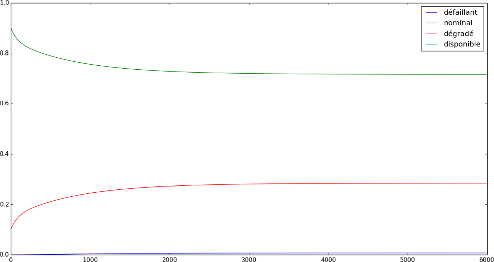
Drawing plots
Now you are able to compute the probabilities you want, for the states you want, for the time you want, let’s plot those probabilities. The following code gives you a example of how to plot the variation of the probabilities.
>>> import pylab as p
>>> states = {u'normal': normal,
...           u'available': available,
...           u'damaged': damaged,
...           u'faulty': faulty,
...          }
>>> timerange = range(0, 6000, 10)
>>> for (name, func) in states.iteritems():
...     proba = [process.value(t, func) for t in timerange]
...     p.plot(timerange, proba, label=name)
>>> p.legend()
>>> p.show()
And, this code gives you the following figure: