How to build a system
A system is built by putting components together. So, let’s have a look on how to build components.
Building components
A component is defined as an instance of the
Component class having a constant reliability rate,
let’s say \(\lambda = 10^{-4}h^{-1}\).
>>> from fiabilipy import Component
>>> from sympy import Symbol
>>> t = Symbol('t', positive=True)
>>> comp = Component('C0', 1e-4)
You have successfully created your first component. C0 is the name of the component ; naming your components will be useful to draw diagrams later.
You can access to some useful information about your component, such as the MTTF, the reliability etc.
>>> comp.mttf
10000.0
>>> comp.reliability(1000)
0.904837418035960
>>> comp.reliability(t)
exp(-0.0001*t)
>>> comp.reliability(t=100)
0.990049833749168
Gather components to build a system
Now you can build components, let’s gather them to build a system. A system is described as a graph of components. There are two special components used to materialize the entry and the exit of the system : E and S. They are compulsory, don’t forget them.
For instance, you could create a simple series system of two components as follow:
>>> from fiabilipy import System
>>> power = Component('P0', 1e-6)
>>> motor = Component('M0', 1e-3)
>>> S = System()
>>> S['E'] = [power]
>>> S[power] = [motor]
>>> S[motor] = 'S'
Once your system is created, you can access to the data you want, such and MTTF, reliability, etc.
>>> S.mttf
1000000/1001
>>> float(S.mttf)
999.000999000999
>>> S.reliability(t)
exp(-1001*t/1000000)
An example of complex system
Let’s build the following system :
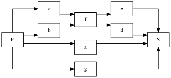
A example of _complex_ system
>>> a, b, c, d, e, f, g = [Component('C%i' % i, 1e-4) for i in xrange(7)]
>>> S = System()
>>> S['E'] = [a, b, c, g]
>>> S[a] = S[g] = S[e] = S[d] = 'S'
>>> S[b] = S[c] = [f]
>>> S[f] = [e, d]
And, you can easily access to the data you want, as previously.
>>> S.mttf
331000/21
>>> S.reliability(t)
13*exp(-t/2000) - 12*exp(-t/2500) - exp(-t/5000) - 6*exp(-3*t/5000) + 2*exp(-t/10000) + 4*exp(-3*t/10000) + exp(-7*t/10000)
As you may see, even if the system is complex, it is quite easy to describe it with fiabilipy.
Draw graphics
Now you know how to build system with ease, let’s draw some graphics. For instance, reliability versus time.
The first thing to do, is to import the pylab module, which provides a
lot of function to do mathematical stuff and to draw graphics:
>>> import pylab as p
Now, let’s define a simple parallel system with two components.
>>> a, b = Component('a', 1e-4), Component('b', 1e-6)
>>> S = System()
>>> S['E'] = [a, b]
>>> S[a] = S[b] = 'S'
In order draw the graphic, we need a time range of study, for instance, from \(t = 0\) to \(t = 200\), by steps of \(10\) (the unit of time is the one you choose). Once the time range is defined, we compute the reliability of each time step:
>>> timerange = range(0, 20000, 100)
>>> reliability = [S.reliability(t) for t in timerange]
To finish, you only have to plot:
>>> p.plot(timerange, reliability)
>>> p.show()
You can admire the result.
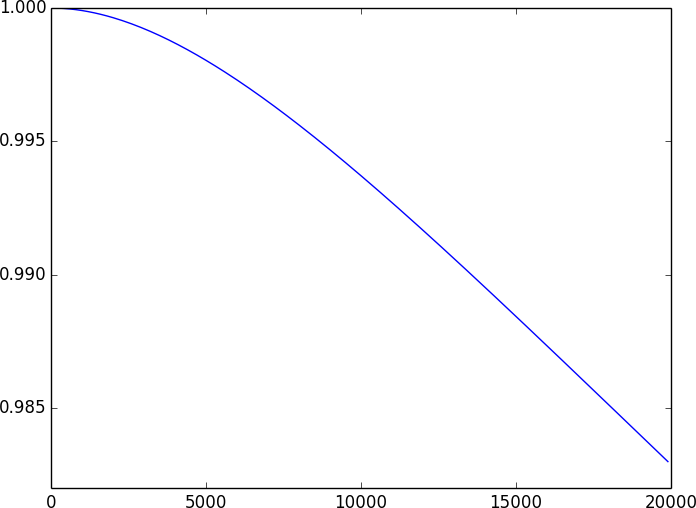
The reliability graphic